Implementation
Computational Implementation
To transform raw tracking coordinates into a functional physics engine, we developed a custom big data pipeline capable of processing spatiotemporal SportVU data at scale.
Data Structure & Schema
Our pipeline ingests raw tracking frames structured as nested arrays. Each “moment” represents a discrete snapshot of the court at a sampling rate of 25 frames per second.
Ball Position (Index 0)
- Team/Player ID: -1
- X / Y: Court Coordinates
- Z: Height of the ball
Player Positions (Indices 1-10)
- Team ID: NBA Team Identifier
- Player ID: Official NBA Player ID
- X / Y: Court Coordinates
- Z: 0.0 (Floor level)
- Data Pipeline & Alignment
Our primary dataset consists of spatiotemporal SportVU tracking data, spanning over 600 games and 90,000 shots from the 2015-2016 NBA season. The system allowed us to structure raw data for high-speed simulations[cite: 42].
True Release Frame Synchronization
Initial data verification revealed a systematic temporal lag (typically 3-4 seconds) in Play-by-Play shot timestamps relative to the physical release of the ball. To evaluate defensive positioning at the moment of peak threat, we developed a trajectory-based alignment protocol.
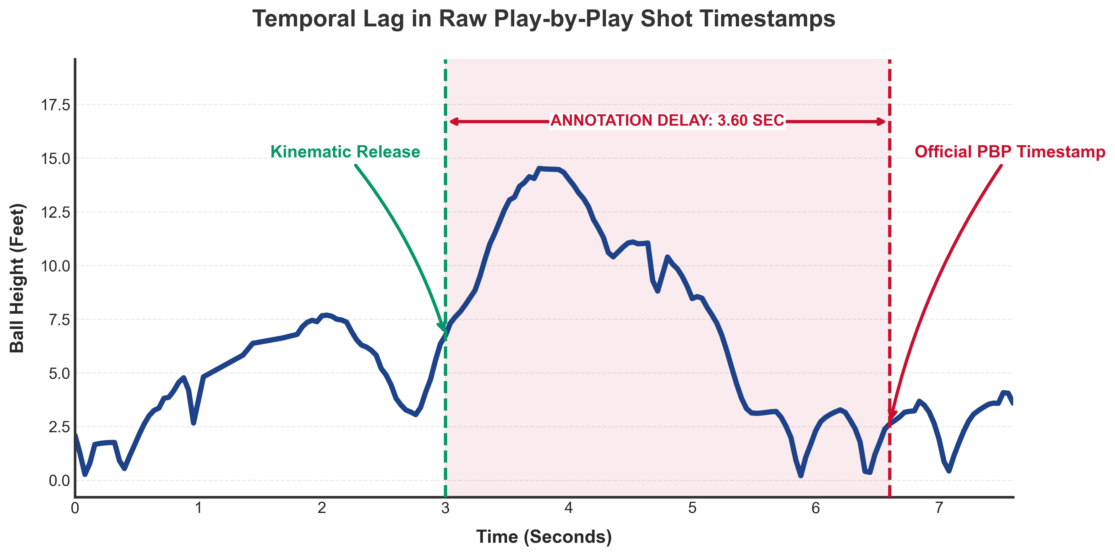
Figure 1: Trajectory-based alignment identifying the "True Release Frame".
By backtracking from the delayed timestamp to the frame where the ball begins its vertical ascent, our pipeline determines the exact defensive configuration at the moment the shot is taken.
- Representing Scoring Threat
Spatial Quality Maps (Q)
Because the JKO scheme requires continuous spatial gradients, we translated discrete shot data into 2D Expected Points Per Shot (xPPS) surfaces. We applied a Gaussian filter (\(\sigma=1.25\)) to create a smooth, differentiable field for the physics engine.
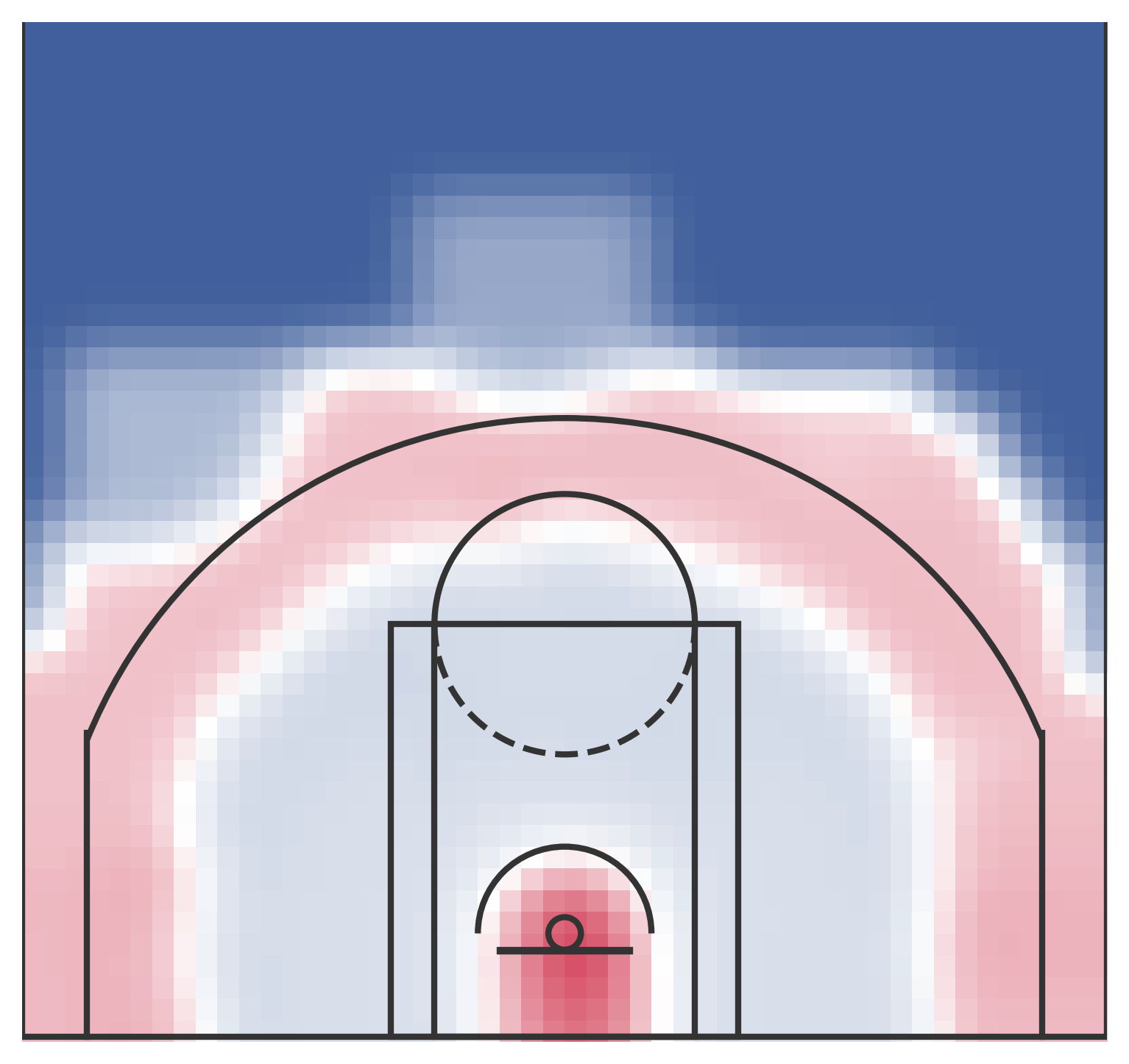
Figure 2a: Versatile Threat (Kawhi Leonard)
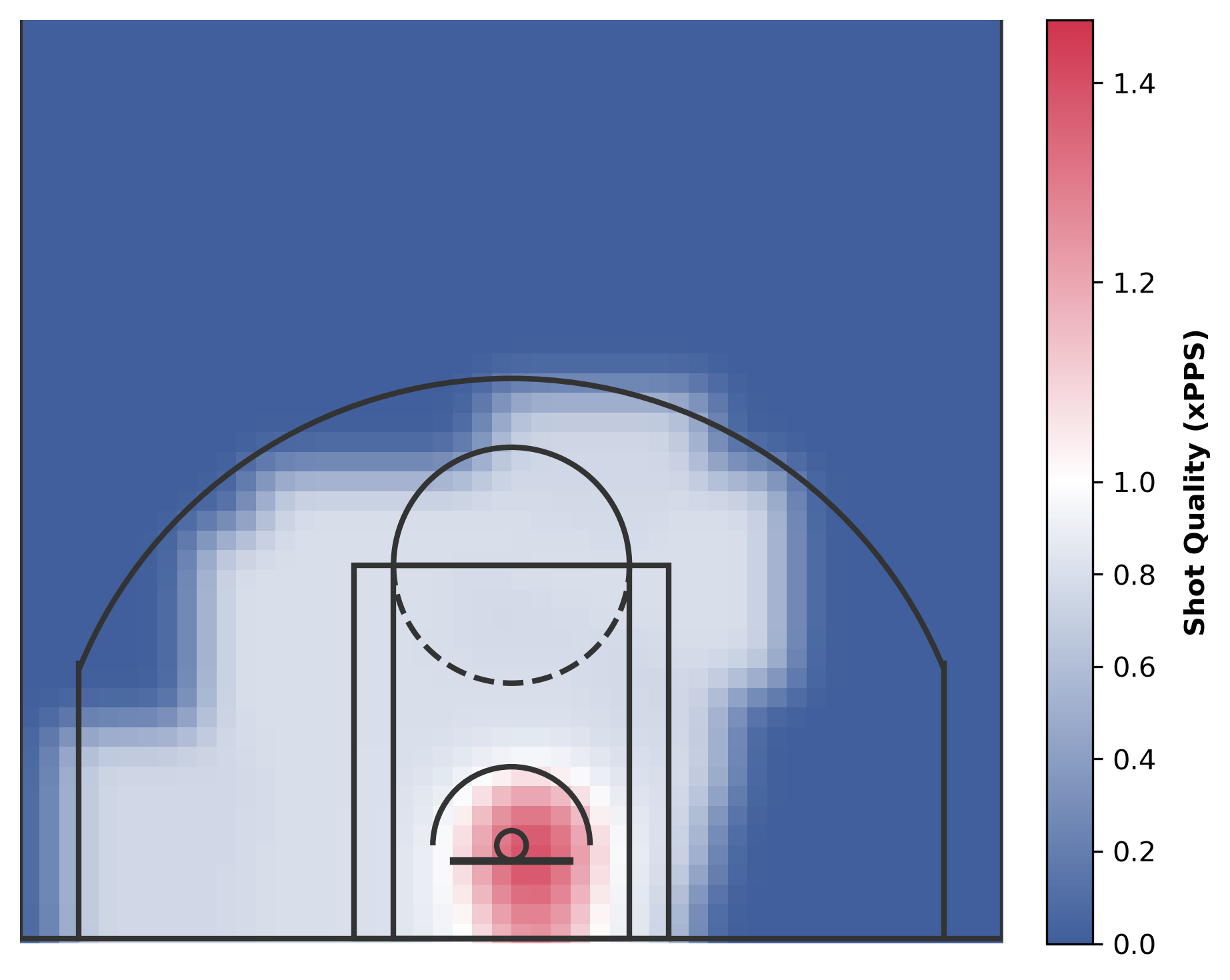
Figure 2b: Rim-Centric Threat (Rudy Gobert)
Instantaneous Shot Threat (IST)
To prioritize threats dynamically, IST is calculated as a multiplicative interaction between Shot Quality (Q), Defensive Openness (O), and Distance to the Ball (B), each weighted by their respective exponents. We established an empirical contest threshold of 4.80 feet.
\[IST = \beta_0 \cdot (Q)^{\beta_Q} \cdot (O)^{\beta_O} \cdot (B)\]
The system utilizes a softmin operator to identify the nearest defender while maintaining a stable gradient for the solver:
\(d_{closest} = -\frac{1}{k_{smooth}} \ln \left( \sum_{p_d \in P_D} e^{-k_{smooth} \cdot \|p_d - p_o\|} \right)\)
- The JKO Solver
The simulation is powered by a solver responsible for calculating defensive movements using JAX and Optimal Transport concepts.
Composite Loss Function
The JKO solver steps the simulation forward by minimizing a composite loss function to find optimal defender positions
\(L_{total} = L_{potential} + L_{kinetic} + L_{acceleration} + L_{velocity}\)
- Kinetic Energy: This term quantifies the cost of moving defenders using the Sinkhorn divergence, a differentiable approximation of the Wasserstein-2 distance.
- Acceleration Penalty: Discourages rapid changes in velocity, making movements more fluid and less vibrating.
- Large-Scale Simulation Pipeline
To evaluate the efficacy of the JKO scheme, we engineered a batch-processing simulation pipeline capable of evaluating thousands of continuous NBA possessions.
For each possession, the pipeline initializes all ten players at the start of the temporal window. While the offensive players follow their real historical trajectories, the defensive players are controlled entirely by the JKO physics engine. The engine calculates the optimal movement for each defender frame-by-frame, allowing the defense to dynamically react to the evolving offensive play.
We ran this batch simulation across the validation and test sets, requiring approximately 6 hours of compute time. To compare results, the pipeline exports three key outputs per possession:
- JKO Defensive Trajectories: The coordinate matrices (\(P_{D,\text{sim}}\)) generated by the JKO solver.
- Real-World Tracking Data: The coordinate matrices (\(P_{D,\text{real}}\)) of the historical NBA defenders.
- Delta Threat Metrics: The frame-by-frame Instantaneous Shot Threat (IST) for both the simulated and real defenses.
Source Code & Data
Explore the full Python implementation and JAX-based solver on our GitHub repository.
View GitHub Repository